Lab 10: Localization (sim)

Goal

The goal of this lab was to localize a virtual robot on a discrete grid using a Bayes filter. The robot state was (x, y, theta), and the map was discretized into 12 x 9 x 18 = 1944 cells. I used the provided simulator, the precomputed map views, and the sample trajectory from the notebook.

Before working on localization, I used the simulator notebook to verify that the robot could follow velocity commands and that the plotter was logging the ground truth and odometry traces correctly. I added an open loop square command to the notebook because it was a quick sanity check before debugging the probabilistic part.

Motion Checks

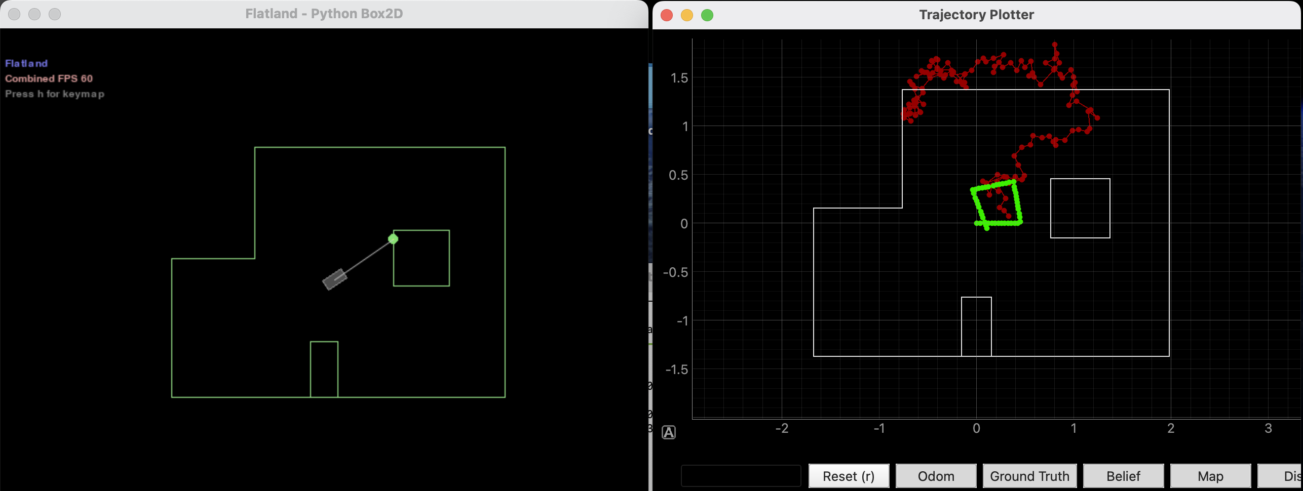
My first square run was not clean. The path drifted upward and the odometry trace spread far outside the small square region. That told me the basic plotting pipeline was working, but the command timing was still rough.

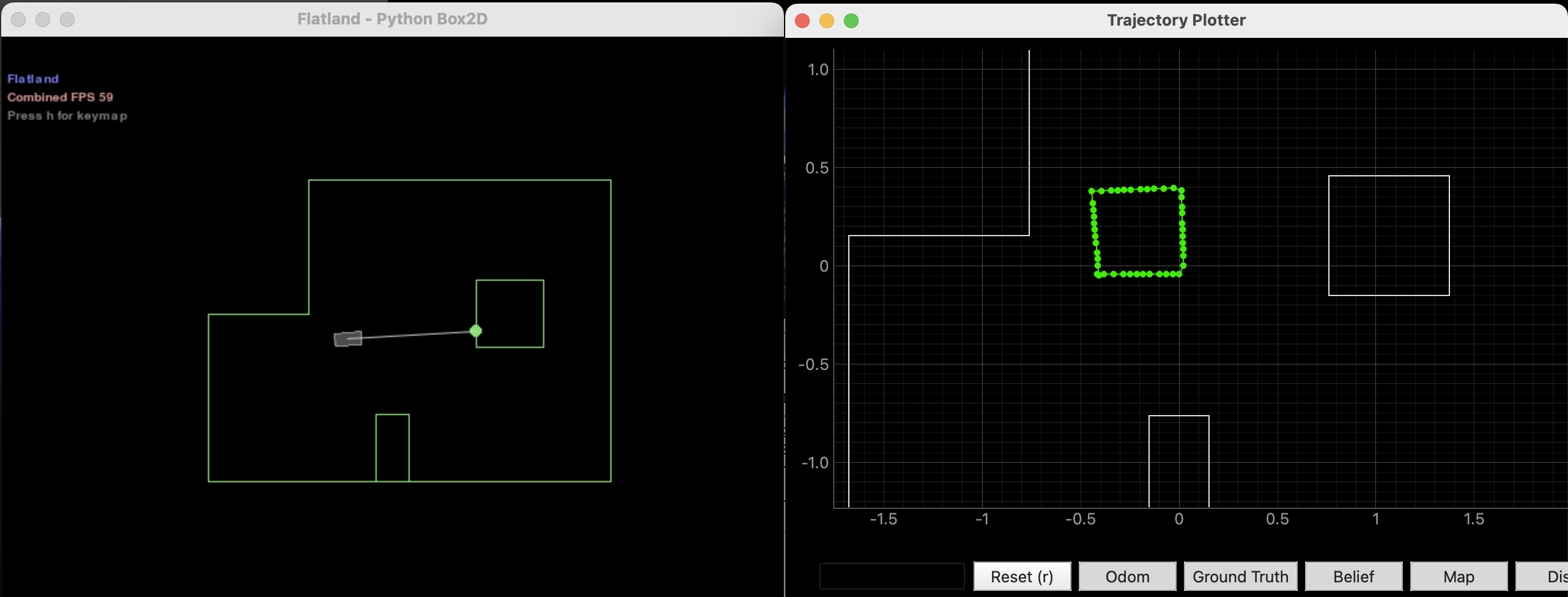
After tuning the forward and turn durations, the open loop square became much tighter. From the plot, the final square side length was about 0.43 m, and the four corners stayed visually consistent. That gave me enough confidence to move on to Bayes filtering.

Bayes Filter Design

I followed the standard two step Bayes filter structure from the lab notebook and the lecture notes.

For the motion model, I used odometry and decomposed each move into rot1, trans, and rot2. compute_control() extracts those three values from the previous and current odometry poses. odom_motion_model() then compares the measured control against the control implied by a candidate state transition. I modeled the error in each term with a Gaussian and multiplied the three likelihoods together.

For the update step, I compared the 18 measured range values from the observation loop against the 18 expected range values stored in mapper.obs_views. Each measurement was scored with a Gaussian sensor model. Then I multiplied the 18 likelihoods to get the observation probability for each state.

I used the same overall analysis style as the report I referenced from the course site: explain the motion model first, then the sensor model, then show how prediction drifts and update pulls the estimate back toward ground truth.

The one implementation choice I changed for speed was the prediction step. I did not use a pure six nested loop version. I kept the useful pruning idea from the reference report, so I skipped old states whose belief was below 1e-4. Then, for each remaining old state, I used the cached mapper.x_values, mapper.y_values, and mapper.a_values arrays to evaluate the transition probability over the entire grid at once with NumPy. I also used a NumPy angle normalization helper because the provided scalar normalize_angle() cannot handle arrays.

Code

BEL_THRESH = 1e-4

def normalize_angles(angles):
    return (np.asarray(angles) + 180.0) % 360.0 - 180.0

def compute_control(cur_pose, prev_pose):
    dx = cur_pose[0] - prev_pose[0]
    dy = cur_pose[1] - prev_pose[1]
    delta_trans = math.hypot(dx, dy)

    if delta_trans < 1e-9:
        delta_rot_1 = 0.0
    else:
        heading = math.degrees(math.atan2(dy, dx))
        delta_rot_1 = mapper.normalize_angle(heading - prev_pose[2])

    delta_rot_2 = mapper.normalize_angle(
        cur_pose[2] - prev_pose[2] - delta_rot_1
    )
    return delta_rot_1, delta_trans, delta_rot_2

def odom_motion_model(cur_pose, prev_pose, u):
    expected_u = compute_control(cur_pose, prev_pose)
    prob_rot_1 = loc.gaussian(
        mapper.normalize_angle(expected_u[0] - u[0]), 0, loc.odom_rot_sigma
    )
    prob_trans = loc.gaussian(
        expected_u[1] - u[1], 0, loc.odom_trans_sigma
    )
    prob_rot_2 = loc.gaussian(
        mapper.normalize_angle(expected_u[2] - u[2]), 0, loc.odom_rot_sigma
    )
    return prob_rot_1 * prob_trans * prob_rot_2

def prediction_step(cur_odom, prev_odom):
    u = compute_control(cur_odom, prev_odom)
    loc.bel_bar.fill(0)

    significant_states = np.argwhere(loc.bel > BEL_THRESH)
    x_grid = mapper.x_values
    y_grid = mapper.y_values
    a_grid = mapper.a_values

    for px, py, pa in significant_states:
        prev_pose = mapper.from_map(px, py, pa)
        dx = x_grid - prev_pose[0]
        dy = y_grid - prev_pose[1]
        trans = np.hypot(dx, dy)

        headings = np.degrees(np.arctan2(dy, dx))
        rot1 = normalize_angles(headings - prev_pose[2])
        rot1 = np.where(trans < 1e-9, 0.0, rot1)
        rot2 = normalize_angles(a_grid - prev_pose[2] - rot1)

        prob = (
            loc.gaussian(normalize_angles(rot1 - u[0]), 0, loc.odom_rot_sigma)
            * loc.gaussian(trans - u[1], 0, loc.odom_trans_sigma)
            * loc.gaussian(normalize_angles(rot2 - u[2]), 0, loc.odom_rot_sigma)
        )
        loc.bel_bar += loc.bel[px, py, pa] * prob

    loc.bel_bar /= np.sum(loc.bel_bar)

def update_step():
    measured = np.asarray(loc.obs_range_data).reshape(1, 1, 1, -1)
    expected = mapper.obs_views
    measurement_prob = loc.gaussian(measured, expected, loc.sensor_sigma)
    sensor_prob = np.prod(measurement_prob, axis=3)

    loc.bel = loc.bel_bar * sensor_prob
    loc.bel /= np.sum(loc.bel)

Results

The initial update step already concentrated the belief strongly. Starting from a uniform prior of 1 / 1944 = 0.0005144 per cell, the update step produced a maximum belief of 0.999995 at grid index (5, 4, 9), while the ground truth index was (6, 4, 9). So after only the first observation loop, the estimate was already one x cell away from the correct state.

Initial grid belief before localization. The prior is uniform over the full map.

Belief after localization. The highest probability region concentrates near the robot trajectory instead of staying spread across the grid.

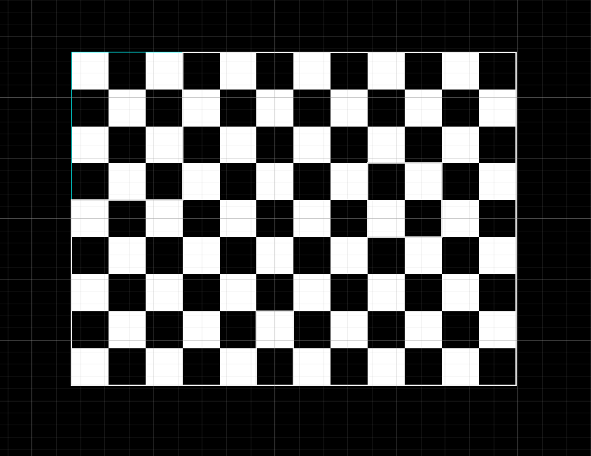
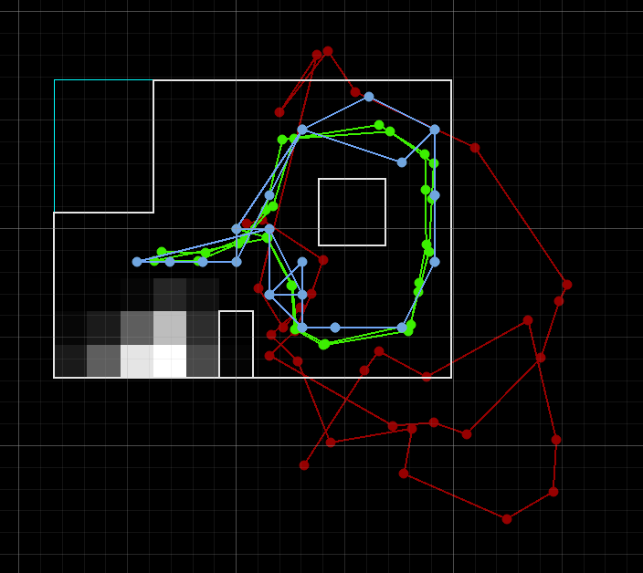
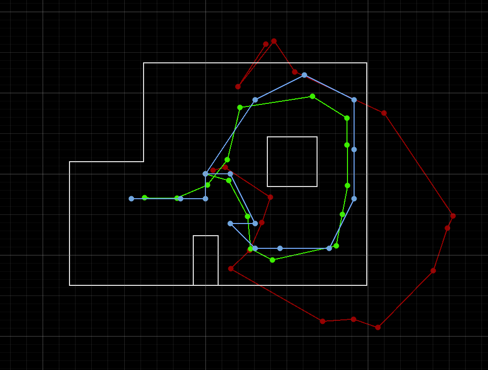
Along the trajectory, the prediction step drifted as expected because it only used noisy odometry. At time step 0, the prior belief maximum was at (1, 5, 12) with probability 0.1004687, which corresponded to a position error of about 1.506 m in x and 0.393 m in y before the update. After the observation update at the same step, the belief maximum moved to (6, 4, 6) with position error about 0.018 m in x and 0.089 m in y. The raw yaw error printed in the notebook looked huge because the log did not normalize the angle difference back to [-180, 180). Interpreted modulo 360, the yaw error at that step was about 9.9 degrees.

The next few steps showed the same pattern. The prior belief spread or drifted to a wrong region, then the observation update pulled the estimate back near the green ground truth trace. From the saved logs:

• Step 1 update error was about 0.205 m in x, 0.083 m in y, and 7.0 degrees in yaw after angle wrap correction.
• Step 2 update error was about 0.100 m in x, 0.222 m in y, and 15.9 degrees in yaw.
• Step 3 update error was about 0.072 m in x, 0.011 m in y, and 4.1 degrees in yaw.

The full trajectory plot below shows the same story visually. Red is odometry, green is ground truth, and blue is the Bayes filter estimate. The blue trajectory stayed much closer to the green one than the red trajectory did, especially after the robot moved away from the start and odometry accumulated large drift.

Discussion

This implementation worked well enough to show the main idea of grid localization. Prediction alone was not reliable. Update alone could not move the state forward. The combination was much better because the prediction step gave a motion prior and the observation step corrected that prior using the map.

The two biggest practical issues were computation cost and angle wrap. Computation cost came from the large number of possible state transitions. Pruning low probability states helped a lot. Vectorizing the sensor update helped even more. Angle wrap mattered because headings like 350 degrees and -10 degrees represent almost the same direction, but a naive Gaussian would treat them as very far apart. The extra NumPy normalization helper fixed that issue in the prediction step.

The result is still not perfect. The estimate snaps to cell centers, so some quantization error is unavoidable. The blue trajectory also deviates more in places where the map geometry is less distinctive or the robot is turning near obstacles. That behavior matches what I expected from a coarse 20 degree angular grid and 0.3048 m position cells.

Meet my cat Mulberry! 🐱