Lab 2: IMU
Set up the IMU
Hardware Connection
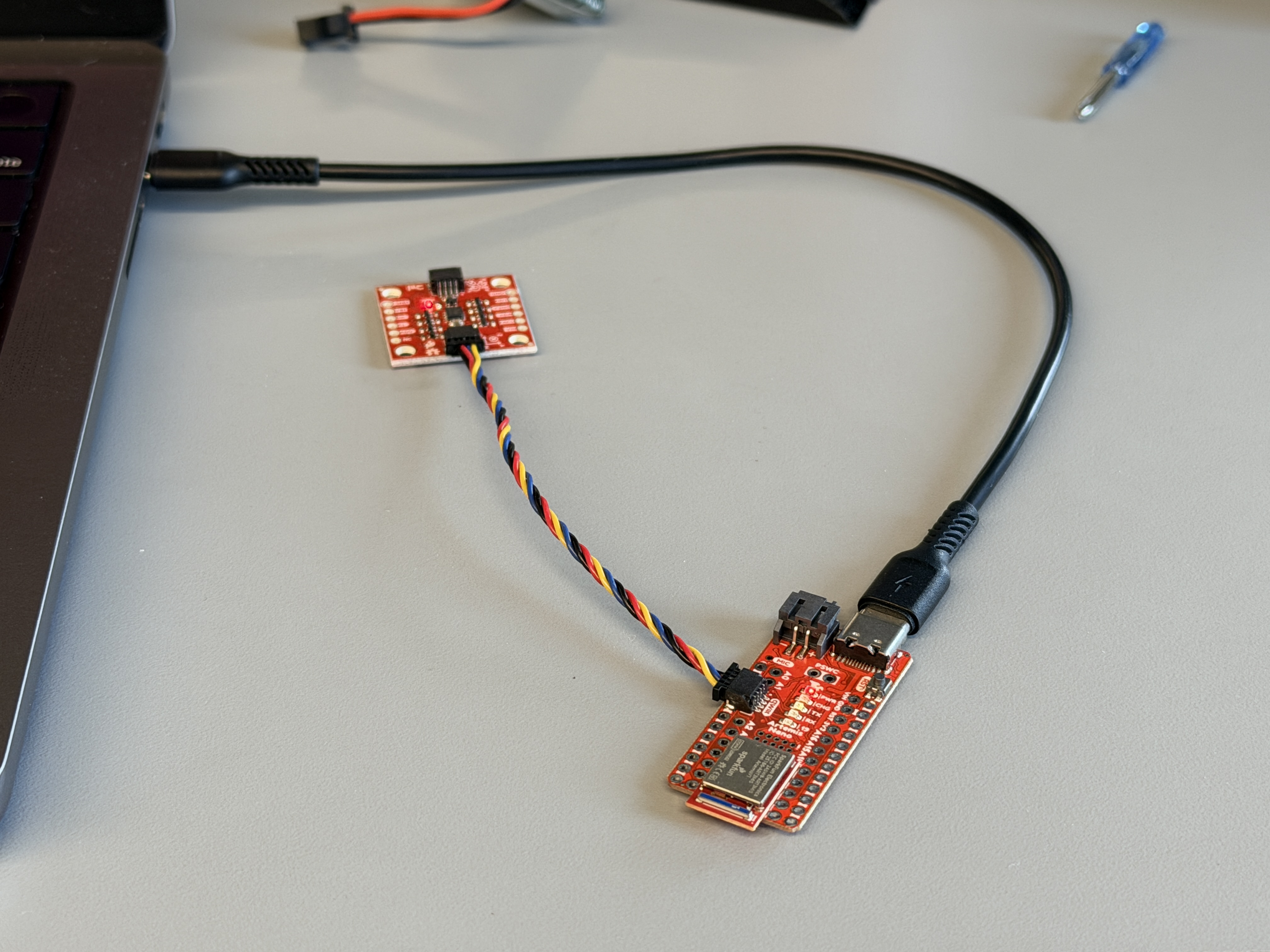
The ICM-20948 9-DOF IMU is connected to Artemis Nano via the QWIIC connector. QWIIC interface supplies 3.3V, GND, SDA and SCL.
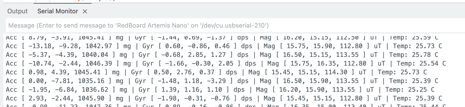
After running the Example1_Basics sketch, the Serial Monitor confirmed successful initialization, and both accelerometer and gyroscope readings updated in real time:
On startup, the LED blinks three times to show the board is running.
Arduino: LED startup blink
// In setup()
for (int i = 0; i < 3; i++) {
    digitalWrite(LED_BUILTIN, HIGH);
    delay(300);
    digitalWrite(LED_BUILTIN, LOW);
    delay(300);
}
AD0_VAL Discussion
AD0_VAL sets the last bit of the ICM-20948 I2C address. If AD0_VAL = 1, the address is 0x69 (ADR jumper open, which is the default). If AD0_VAL = 0, the address is 0x68 (ADR jumper closed). This is useful if two ICM-20948 sensors share one I2C bus, since each sensor can use a different address. In this lab I only used one IMU, so I left the ADR jumper open and used AD0_VAL = 1.
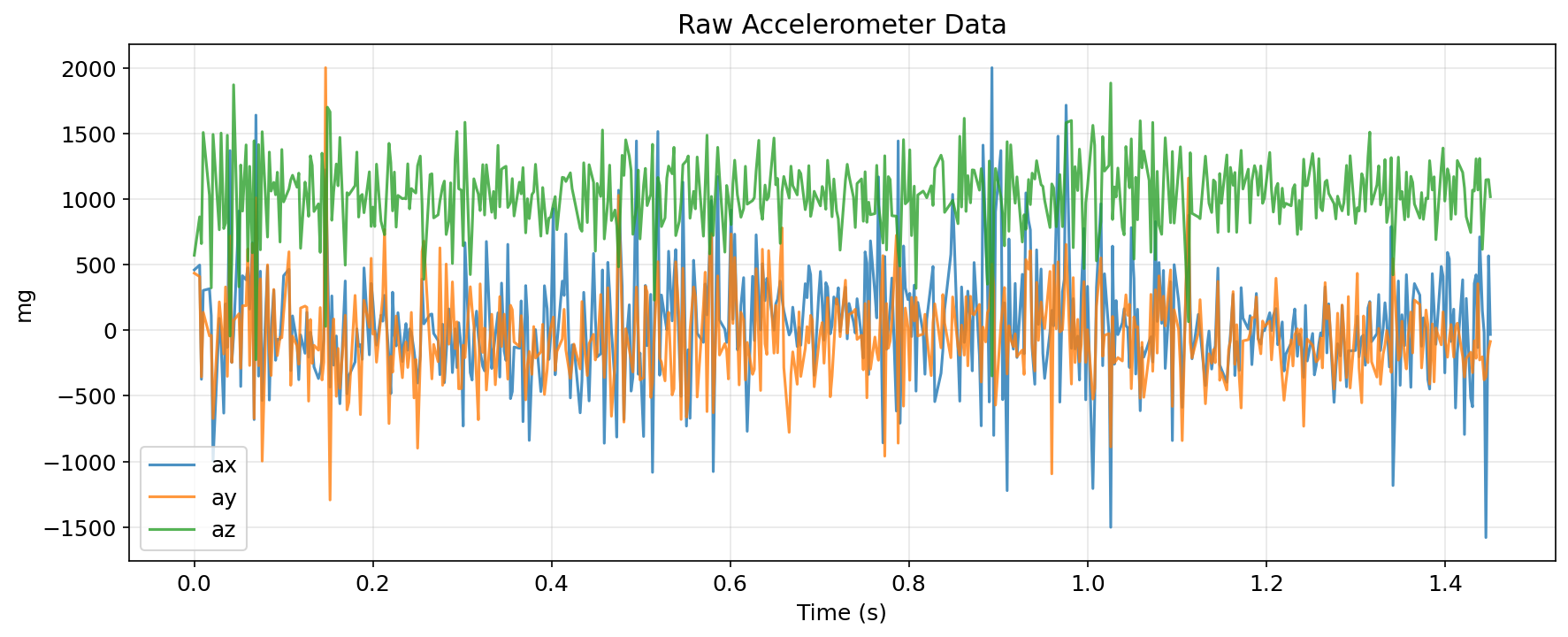
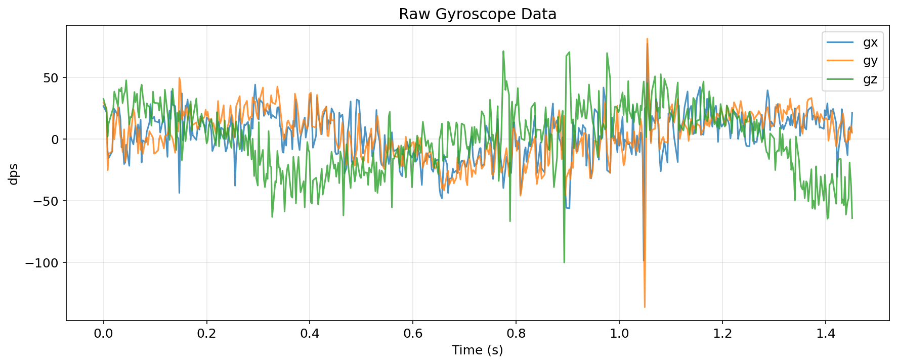
Accelerometer and Gyroscope Data
When rotating or flipping the board, the accelerometer X/Y/Z readings change to reflect the component of gravity projected onto each axis. At rest flat on a table, az ≈ 1000 mg while ax and ay approach 0. Rotating 90° about the X-axis causes ay to swing from 0 to ±1000 mg. The gyroscope outputs angular velocity (dps) on each axis. Rapid accelerations produce large transient spikes in the accelerometer, while slow steady tilts show up clearly in the gyroscope as sustained non-zero readings.
Accelerometer
Pitch and Roll Calculation
Pitch and roll are derived from accelerometer gravity projection using:
\[\text{pitch} = \arctan\!\left(\frac{a_x}{\sqrt{a_y^2 + a_z^2}}\right) \times \frac{180}{\pi}\] \[\text{roll} = \arctan\!\left(\frac{a_y}{\sqrt{a_x^2 + a_z^2}}\right) \times \frac{180}{\pi}\]Using atan2 (from math.h) avoids quadrant ambiguity and handles the case where the denominator approaches zero.
Arduino: pitch and roll from accelerometer
#include <math.h>

float ax = myICM.accX();  // mg
float ay = myICM.accY();
float az = myICM.accZ();

float pitch_a = atan2(ax, sqrt(ay*ay + az*az)) * 180.0 / M_PI;
float roll_a  = atan2(ay, sqrt(ax*ax + az*az)) * 180.0 / M_PI;
Output at -90, 0, 90 Degrees
Measurements at the three reference orientations, taken as the mean of 10 consecutive readings:
| Orientation | Pitch (measured) | Roll (measured) |
|---|---|---|
| 0° (flat) | -2.68° | -0.63° |
| +90° | 86.23° | 86.09° |
| -90° | -89.05° | -85.51° |
The accelerometer reads close to 90° but not exactly because achieving a perfect right-angle by hand is difficult. The flat (0°) reading shows a small offset bias of about -2.7° for pitch and -0.6° for roll.
Accelerometer Accuracy and Two-Point Calibration
A two-point calibration was performed using the ±90° measurements as reference endpoints. The calibration computes a linear scale and offset such that the corrected output matches the expected output:
\[\text{corrected} = \text{scale} \times \text{measured} + \text{offset}\]For pitch, the fitted values were scale = 1.027 and offset = +1.45°. For roll, they were scale = 1.049 and offset = −0.31°.
After calibration, errors at the extreme angles are reduced to < 1°. The remaining error at 0° is within the expected bias of a consumer-grade MEMS sensor.
Python: two-point calibration function
def two_point_calibration(measured_low, measured_high,
                           expected_low=-90.0, expected_high=90.0):
    scale  = (expected_high - expected_low) / (measured_high - measured_low)
    offset = expected_high - scale * measured_high
    print(f"Scale: {scale:.6f}, Offset: {offset:.4f}")
    return scale, offset

# Pitch: measured -89.05 at -90, 86.23 at +90
pitch_scale, pitch_offset = two_point_calibration(-89.05, 86.23)
# Roll: measured -85.51 at -90, 86.09 at +90
roll_scale, roll_offset   = two_point_calibration(-85.51, 86.09)
Noise and Frequency Spectrum Analysis
FFT analysis was performed on stationary accelerometer pitch data (sampling rate ≈ 342.7 Hz, Nyquist ≈ 171.4 Hz):
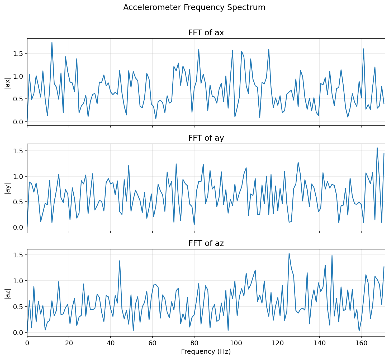
In the stationary case, noise energy is concentrated below 10 Hz with no strong peaks, the sensor is well-behaved at rest. To induce vibration noise, the table was tapped gently during a second recording:
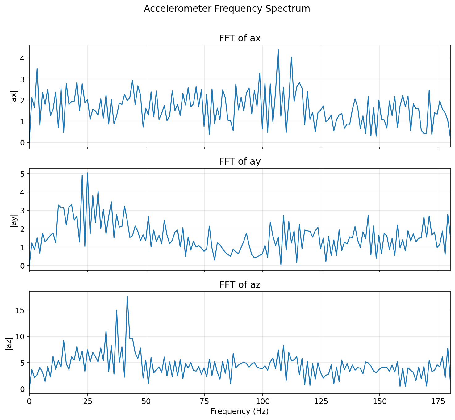
Tapping the table introduces broadband noise spanning multiple frequency bands. The useful orientation signal (slow tilts) lives below ~5 Hz, while the vibration energy appears primarily above 10 Hz. This motivates a low-pass filter with a cutoff in the 5–10 Hz range.
Python: FFT analysis
import numpy as np
import matplotlib.pyplot as plt

def plot_fft(df, col, title=None):
    sig = df[col].values
    n   = len(sig)
    dt  = np.mean(np.diff(df['time_s'].values))
    fs  = 1.0 / dt

    fft_vals   = np.fft.rfft(sig - np.mean(sig))
    freqs      = np.fft.rfftfreq(n, d=dt)
    magnitudes = np.abs(fft_vals) * 2.0 / n

    plt.figure(figsize=(10, 4))
    plt.plot(freqs, magnitudes)
    plt.xlabel('Frequency (Hz)')
    plt.ylabel('Magnitude')
    plt.title(title or f'FFT of {col}')
    plt.grid(True, alpha=0.3)
    plt.xlim(0, fs/2)
    plt.tight_layout()
    plt.show()
    print(f"Sample rate: {fs:.1f} Hz,  Nyquist: {fs/2:.1f} Hz")
Low-Pass Filter Implementation
The discrete first-order IIR low-pass filter is:
\[y[n] = \alpha \cdot x[n] + (1 - \alpha) \cdot y[n-1], \quad \alpha = \frac{d_t}{d_t + \frac{1}{2\pi f_c}}\]The alpha value for several candidate cutoff frequencies (at the measured 2.92 ms sample period):
| Cutoff Frequency | Alpha |
|---|---|
| 1 Hz | 0.018 |
| 2 Hz | 0.035 |
| 5 Hz | 0.084 |
| 10 Hz | 0.155 |
| 20 Hz | 0.268 |
Selected: α = 0.2 (≈ 10 Hz cutoff). This removes the high-frequency vibration noise visible in the FFT while preserving the full dynamic range of typical orientation changes (< 5 Hz). A lower cutoff (e.g., 1 Hz) would add visible lag during fast tilts; a higher cutoff (e.g., 20 Hz) would leave more vibration noise.
Arduino: low-pass filter on accelerometer pitch/roll
float alpha_lpf = 0.2;  // ~10 Hz cutoff
// Persistent state
float pitch_a_lpf = 0.0, roll_a_lpf = 0.0;

pitch_a_lpf = alpha_lpf * pitch_a + (1.0 - alpha_lpf) * pitch_a_lpf;
roll_a_lpf  = alpha_lpf * roll_a  + (1.0 - alpha_lpf) * roll_a_lpf;
Gyroscope
Pitch, Roll, and Yaw from Gyroscope Integration
The gyroscope outputs angular velocity (dps), so integrating over time gives angle estimates:
\[\theta[n] = \theta[n-1] + \omega \cdot d_t\]In this implementation, pitch (rotation about Y) is integrated from gyrX(), roll (rotation about X) from gyrY(), and yaw (rotation about Z) from gyrZ().
Arduino: gyroscope angle integration
float gx = myICM.gyrX();  // dps
float gy = myICM.gyrY();
float gz = myICM.gyrZ();

unsigned long now = millis();
float dt = (now - lastIMUTime) / 1000.0;
if (dt <= 0) dt = 0.001;  // guard against zero division
lastIMUTime = now;

pitch_g += gx * dt;
roll_g  += gy * dt;
yaw_g   += gz * dt;
Comparison with Accelerometer
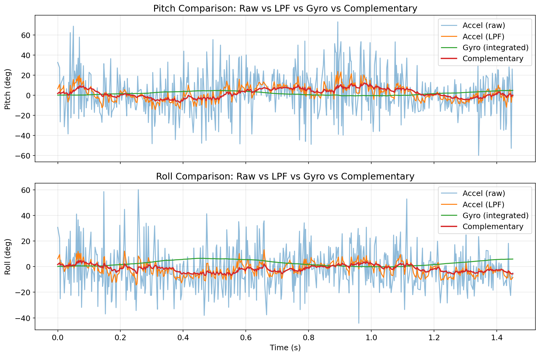
From the comparison plot, the tradeoff is pretty clear. Gyro integration reacts quickly and captures fast motion well, but it drifts over time because bias gets accumulated. The raw accelerometer does not drift, but it gets noisy when the table is tapped or when motion is abrupt, and it cannot provide yaw. The low-pass filtered accelerometer is cleaner, but that filtering also introduces lag. Sampling rate matters a lot for the gyro result: when the rate is reduced, dt gets larger and integration error grows faster. At about 343 Hz, the gyro angle is reliable for short windows (around 10 seconds). At 50 Hz, the error for a fast turn (like 180°/s) is much larger, roughly seven times worse than at 343 Hz.
Complementary Filter
The complementary filter fuses the two sensors — using the gyroscope for short-term accuracy and the accelerometer for long-term correction:
\[\theta[n] = (1-\alpha)\bigl(\theta[n-1] + \omega \cdot d_t\bigr) + \alpha \cdot \theta_\text{accel}\]Arduino: complementary filter
float alpha_comp = 0.05;  // 5% accel weight, 95% gyro weight
float pitch_comp = 0.0, roll_comp = 0.0;

pitch_comp = (1.0 - alpha_comp) * (pitch_comp + gx * dt) + alpha_comp * pitch_a;
roll_comp  = (1.0 - alpha_comp) * (roll_comp  + gy * dt) + alpha_comp * roll_a;
Drift test — IMU held stationary for ~10 seconds:
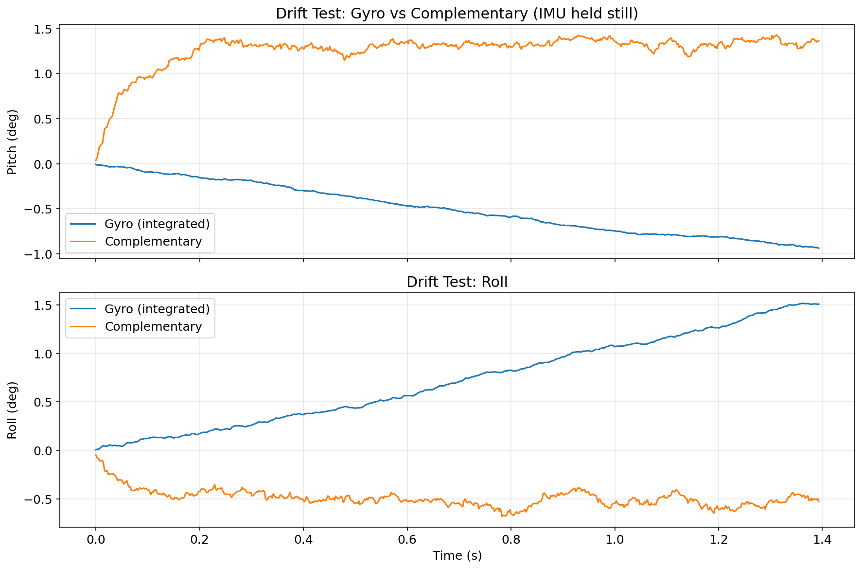
The gyro integral drifts continuously; the complementary filter stays within ~1° of the true angle because the 5% accelerometer weighting slowly corrects any accumulated bias.
Vibration rejection test — table tapped while recording:
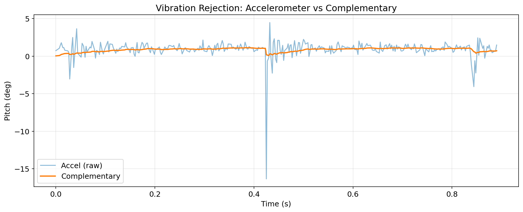
The raw accelerometer spikes by several degrees during each tap. The complementary filter’s dominant gyroscope weight (95%) suppresses these transients, maintaining a smooth output.
For this lab, I used α_comp = 0.05, which gave a good balance between drift correction and vibration rejection. I also kept α_lpf = 0.2 so the accelerometer signal entering the complementary filter was less sensitive to high-frequency shocks. The sample rate stayed around 343 Hz, which was fast enough to capture aggressive motion without large integration error.
Sample Data
Speed of Sampling
With all Serial.print statements and delay() calls removed from the main loop, the Artemis checks myICM.dataReady() on every iteration and stores data only when a new sample is available. The measured throughput is ~343 samples/second (~2.9 ms/sample).
The Artemis main loop runs faster than the IMU’s internal ODR (Output Data Rate). dataReady() returns false on most loop iterations, so the loop does not block — it just polls and moves on. This non-blocking design is critical: the same loop simultaneously handles BLE read_data() without introducing timing jitter.
Arduino: non-blocking main loop
void loop() {
    BLEDevice central = BLE.central();
    if (central) {
        while (central.connected()) {
            write_data();   // period heartbeat
            read_data();    // handle any incoming BLE commands

            // Non-blocking IMU collection only store when data is ready
            if (collectingIMU) {
                record_imu_data();  // returns immediately if !dataReady()
            }
        }
    }
}

void record_imu_data() {
    if (!imuInitialized || imuArrayFull) return;
    if (!myICM.dataReady()) return;  // non-blocking check

    myICM.getAGMT();
    // ... compute angles, store in arrays ...
}
Data Storage Design
Separate arrays are used for each quantity rather than a single large interleaved array. This makes indexing clear and avoids struct padding/alignment overhead:
#define MAX_IMU_SIZE 2000

unsigned long imuTimeStamps[MAX_IMU_SIZE];   // 8 kB
float imuPitchA[MAX_IMU_SIZE];               // 8 kB
float imuRollA[MAX_IMU_SIZE];                // 8 kB
float imuPitchALpf[MAX_IMU_SIZE];            // 8 kB
float imuRollALpf[MAX_IMU_SIZE];             // 8 kB
float imuPitchG[MAX_IMU_SIZE];               // 8 kB
float imuRollG[MAX_IMU_SIZE];                // 8 kB
float imuYawG[MAX_IMU_SIZE];                 // 8 kB
float imuPitchComp[MAX_IMU_SIZE];            // 8 kB
float imuRollComp[MAX_IMU_SIZE];             // 8 kB
// Total 2000 samples: ~80 kB
I used float (4 bytes) for stored angle data. The angle range is about −180° to +180°, and I still needed fractional precision, so int16_t felt too limiting. double would double memory use without a real accuracy benefit for this sensor noise level. The Artemis has 384 kB RAM, and these IMU arrays use about 80 kB. After accounting for code, stack, and BLE buffers, there is still enough room for data logging. With all fields stored, capacity is around 3900 samples (about 11.4 s at 343 Hz). If only the compact 5-field format is kept, capacity is roughly 12,500 samples (about 36 s at 343 Hz).
5+ Seconds of IMU Data via Bluetooth
After recording, the SEND_IMU_DATA command transmits the stored data. To stay within BLE bandwidth limits, every 3rd sample is sent (downsampling to ~115 Hz effective), with a 30 ms delay between packets to prevent buffer overflow:
Arduino: SEND_IMU_DATA command
case SEND_IMU_DATA:
{
    int limit = imuArrayFull ? MAX_IMU_SIZE : imuIndex;
    int step  = 3;  // downsample ~115 Hz effective

    for (int i = 0; i < limit; i += step) {
        tx_estring_value.clear();
        tx_estring_value.append((int)imuTimeStamps[i]);
        tx_estring_value.append("|");
        tx_estring_value.append(imuPitchA[i]);
        tx_estring_value.append("|");
        tx_estring_value.append(imuRollA[i]);
        tx_estring_value.append("|");
        tx_estring_value.append(imuPitchComp[i]);
        tx_estring_value.append("|");
        tx_estring_value.append(imuRollComp[i]);
        tx_characteristic_string.writeValue(tx_estring_value.c_str());
        delay(30);  // throttle to prevent BLE buffer overflow
    }
    break;
}
Python: notification handler and data collection
imu_data_buffer = []

def imu_notification_handler(sender, data):
    msg = data.decode('utf-8')
    imu_data_buffer.append(msg)

def collect_imu_data(duration_s=5):
    global imu_data_buffer
    imu_data_buffer = []

    ble.start_notify(ble.uuid['RX_STRING'], imu_notification_handler)
    ble.send_command(CMD.START_IMU_RECORDING, "")
    time.sleep(duration_s)
    ble.send_command(CMD.STOP_IMU_RECORDING, "")
    time.sleep(0.5)
    ble.send_command(CMD.SEND_IMU_DATA, "")

    # wait for transfer to complete
    time.sleep(duration_s * 0.035 * 100 + 5)
    ble.stop_notify(ble.uuid['RX_STRING'])

    # parse pipe-delimited format: time_ms|pitch_a|roll_a|pitch_comp|roll_comp
    rows = []
    for line in imu_data_buffer:
        parts = line.split('|')
        if len(parts) == 5:
            try:
                rows.append([float(x) for x in parts])
            except ValueError:
                pass
    return pd.DataFrame(rows,
        columns=['time_ms', 'pitch_a', 'roll_a', 'pitch_comp', 'roll_comp'])
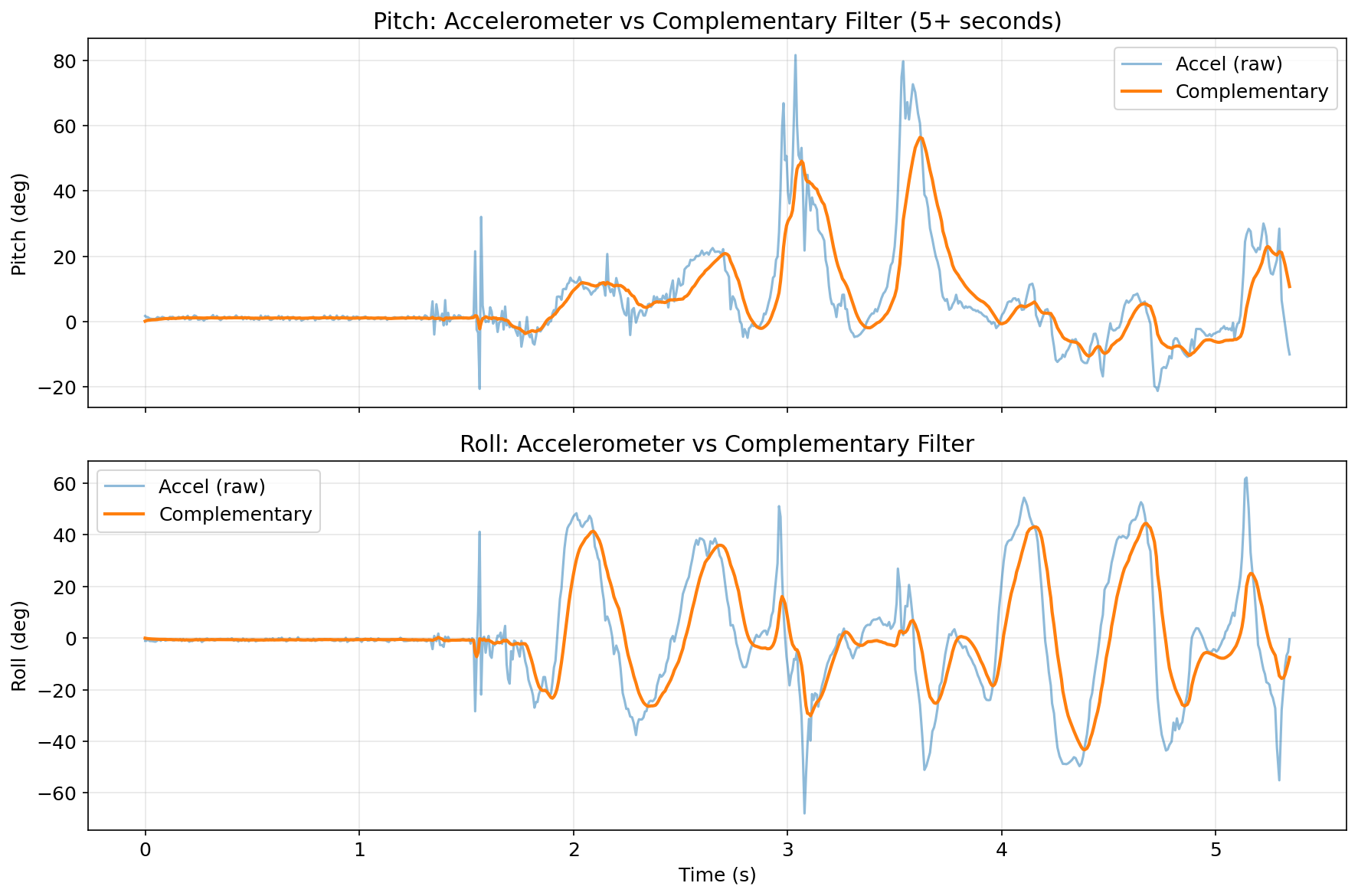
Successfully transmitted 5.34 seconds of IMU data over BLE (667 samples at an effective 124.8 Hz):
Record a Stunt
Stunt 1: Drift and backhit
Stunt 2: Turning
Stunt 3: Flips
The car accelerates hard from rest and has a noticeable forward lurch at full throttle. At higher speed, turning often causes sideways drift, especially on smooth floors. It can also flip end-over-end with a quick reverse input. From these tests, the main takeaway is that the IMU has to deal with sharp transients and vibration-heavy motion, so a gyro-dominant complementary filter is important for keeping the angle estimate stable.
Discussion
Method Comparison and Takeaways
Across all tests, the raw accelerometer worked well as an absolute reference when the system was mostly static, but it became noisy during vibration and of course could not provide yaw. The LPF version improved that noise issue, but lag became noticeable when motion was faster. Gyroscope integration gave the best short-term motion tracking and captured yaw, but drift accumulated if I let it run too long without correction. The complementary filter gave the best overall behavior in this lab: it stayed responsive during motion while still correcting long-term drift.
The biggest practical lesson was that communication limits were more restrictive than sensing limits. The IMU could sample around 343 Hz, but BLE throughput was much lower, so local buffering plus delayed batch transfer was necessary. The non-blocking loop structure also mattered a lot, because it let BLE command handling and IMU logging run together without stalling each other.
Meet with my cat Mulberry! 🐱