Lab 7: Kalman Filter

Goal: build a Kalman Filter that replaces linear extrapolation for the wall-approach PID controller. The filter runs on the Artemis and fills in distance estimates between slow ToF readings so the robot can move faster and more reliably.

KF Equations

I used the standard linear KF equations in both Python and on the Artemis:

x_dot = A_c x + B_c u
y = C x

A_d = I + dt A_c
B_d = dt B_c

mu_p = A_d mu + B_d u
Sigma_p = A_d Sigma A_d^T + Sigma_u

K = Sigma_p C^T (C Sigma_p C^T + Sigma_z)^(-1)
mu = mu_p + K (y - C mu_p)
Sigma = (I - K C) Sigma_p

Step Response and System Identification

I drove the robot at a constant PWM of 80 toward the wall and logged ToF distance at every sensor sample. The firmware stops automatically when distance drops below 500 mm and streams the data back over BLE. I got 18 readings over about 1.5 seconds.

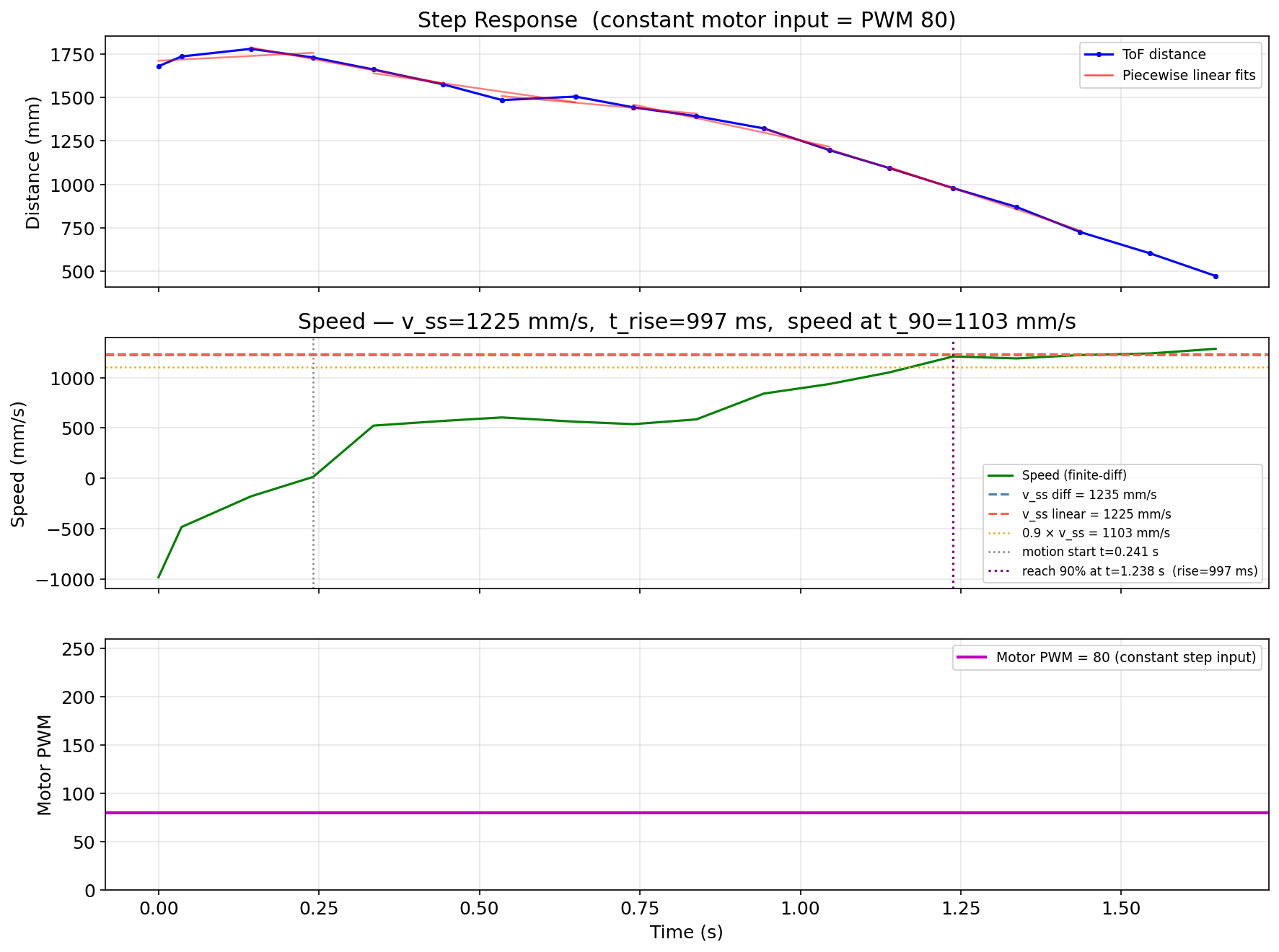
The top panel overlays piecewise linear fits on the raw distance data to show where the slope was measured. The bottom panel confirms the motor input was a constant step at PWM 80 throughout the run. From the velocity curve I extracted two estimates of steady-state speed. The finite-difference method gave 1235 mm/s, and piecewise linear fitting across 50%-overlap segments gave 1225 mm/s. They agree to within 1%, so I used the piecewise-linear result since it is less sensitive to noise spikes at individual ToF samples.

The robot first started moving at t = 0.241 s, reached 90% of v_ss at t = 1.238 s, giving a rise time of 997 ms. The speed at that 90% point was 1103 mm/s. From those three numbers:

v_ss = 1225 mm/s    →  d = 1/v_ss  = 0.000816  s/mm
t_90 = 997 ms       →  m = d × t_90 / ln(10) = 0.000353  s²/mm

Kalman Filter Setup

The continuous-time state space model is:

A_c = [[0,    -1  ],      B_c = [[0       ],      C = [[1, 0]]
       [0,   -d/m ]]             [1/m     ]]

State is [distance, velocity]. C measures distance directly with a positive sign because the ToF reads positive values as the robot approaches.

I computed the actual PID loop period from real timestamps instead of guess: dt = (t_max - t_min) / (N-1), which gave 7.60 ms. Hardcoding 20 ms would have degraded the Ad and Bd accuracy by 2.6x.

Euler discretization:

Ad = I + dt × A_c     Bd = dt × B_c

The initial state is x0 = [first_ToF_reading, 0]^T. Position is set to the first measured distance so the filter starts where the robot actually is. Velocity is set to 0 because the robot has not moved yet at the moment of initialization. The initial covariance is set to Sigma_u so the filter starts with the same uncertainty as one prediction step.

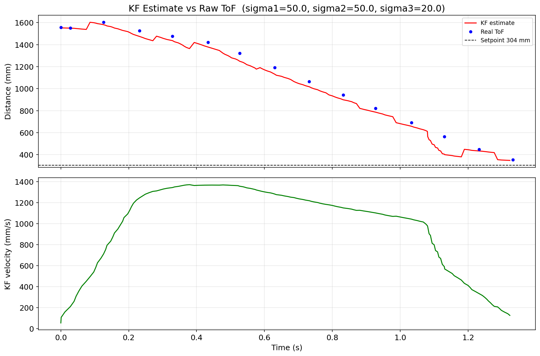
For the covariance matrices I set sigma1 = 50 mm, sigma2 = 50 mm/s, sigma3 = 20 mm. sigma1 and sigma2 are the standard deviations I assume for the model’s position and velocity uncertainty per step. sigma3 is the ToF measurement noise. With these values the filter weighs model predictions and sensor readings roughly equally.

KF Validation in Python

Before putting the filter on the robot, I ran it offline over a separate PID data set. The KF loop steps through every PID timestamp. When a real ToF reading falls within 50 ms of the current PID timestamp, the filter runs prediction + update. Otherwise it runs prediction only.

def kf(mu, sigma, u, y=None):
    mu_p    = Ad.dot(mu) + Bd.dot([[u]])
    sigma_p = Ad.dot(sigma.dot(Ad.T)) + Sigma_u
    if y is None:
        return mu_p, sigma_p
    sigma_m = C.dot(sigma_p.dot(C.T)) + Sigma_z
    K       = sigma_p.dot(C.T.dot(np.linalg.inv(sigma_m)))
    mu      = mu_p + K.dot([[y]] - C.dot(mu_p))
    sigma   = (np.eye(2) - K.dot(C)).dot(sigma_p)
    return mu, sigma

tof_idx = 0
for _, pid_row in pid_sorted.iterrows():
    t_ms = pid_row['time_ms']
    u    = pid_row['motor_pwm'] / STEP_PWM
    y    = None
    if tof_idx < len(real_tof):
        if abs(real_tof['time_ms'].iloc[tof_idx] - t_ms) < 50:
            y = real_tof['dist_mm'].iloc[tof_idx]
            tof_idx += 1
    mu, sigma = kf(mu, sigma, u, y)

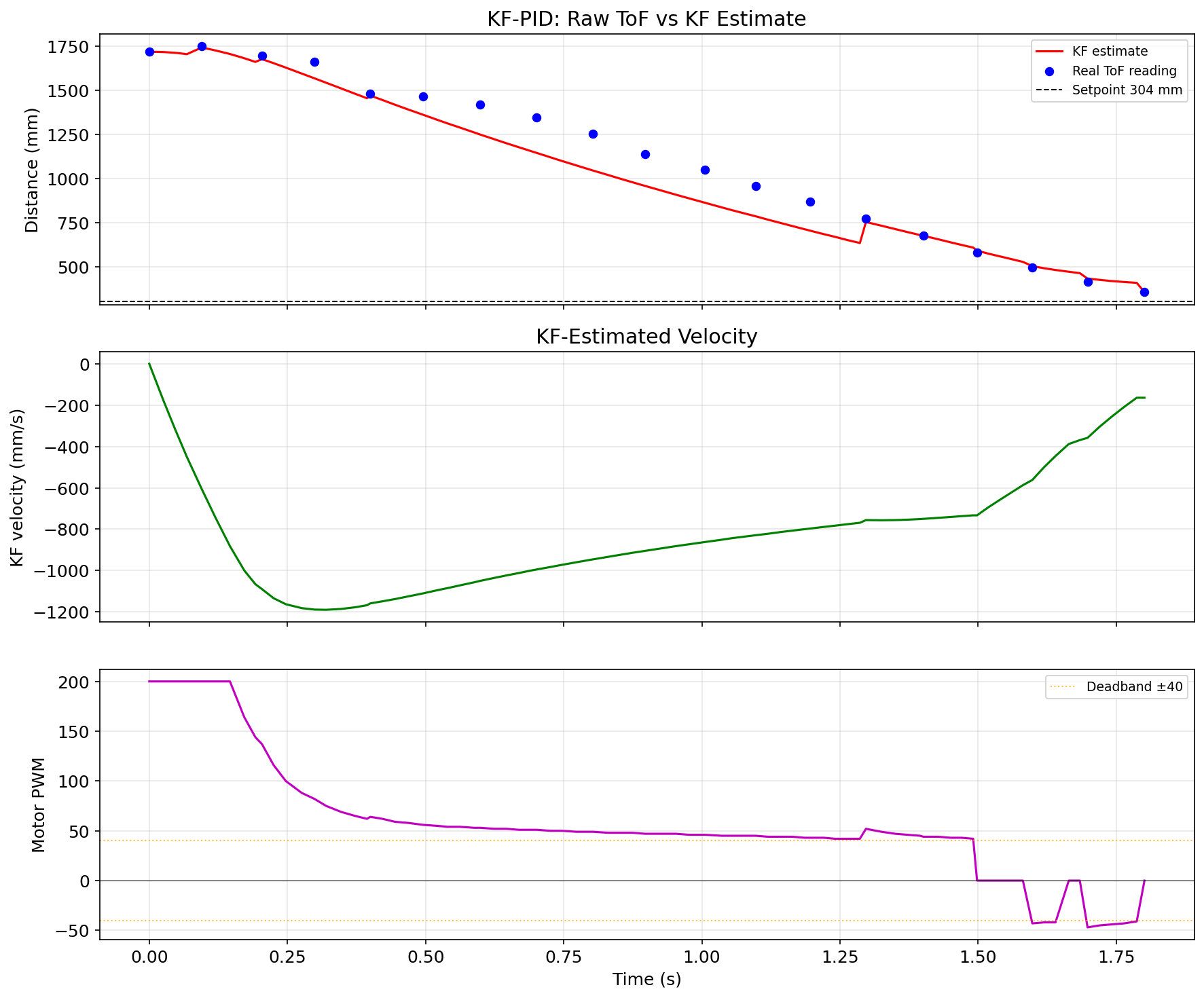
The estimate tracks the raw ToF readings closely and produces a smooth velocity signal that is not available from the sensor alone.

I also compared three sigma configurations to understand the trade-off:

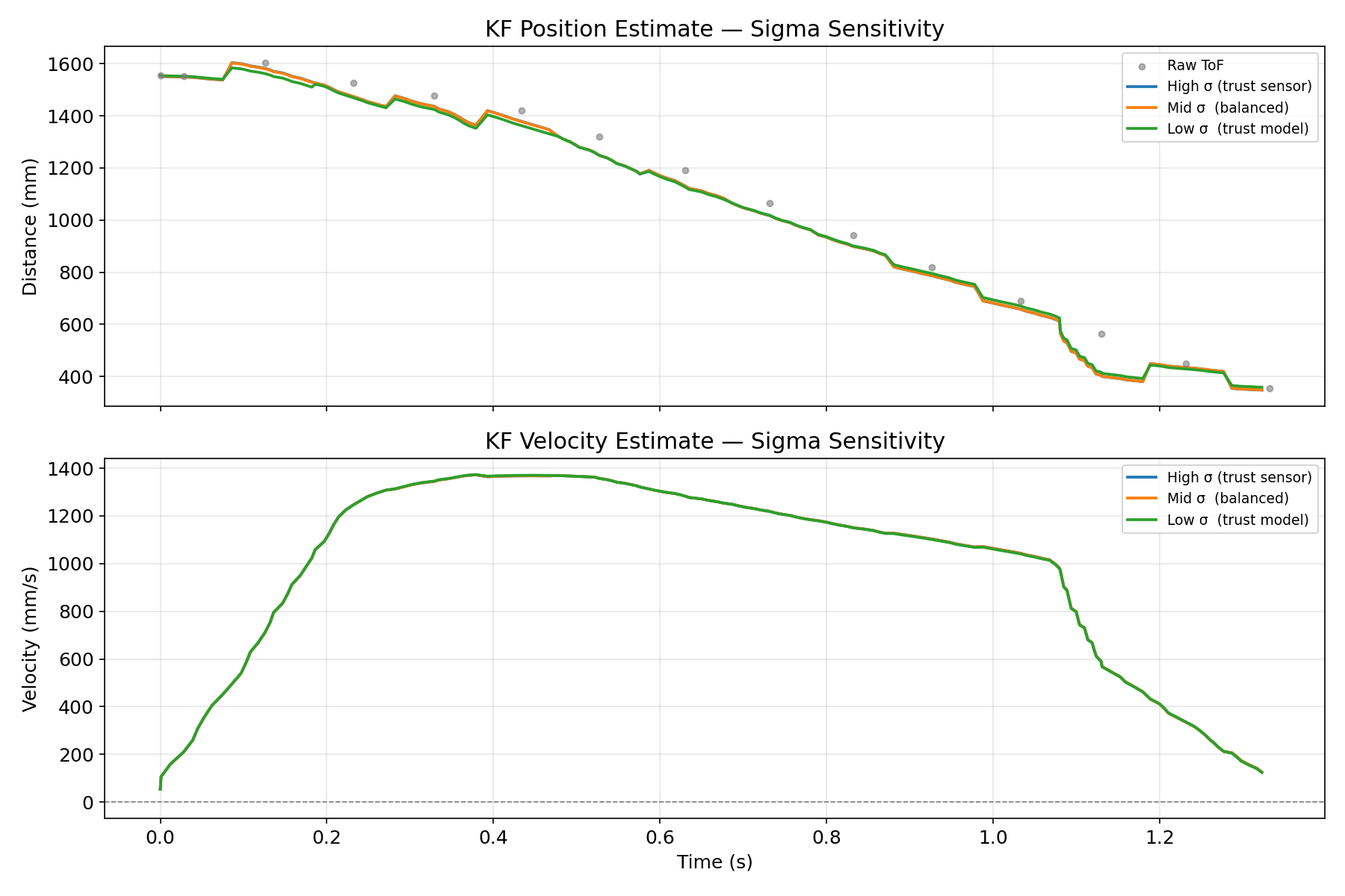
This cannot really see from the figure since the difference are not that huge, but based on result I read: High process noise (sigma1=sigma2=500) makes the estimate chase every measurement closely. Low process noise (sigma1=sigma2=10) locks onto the model and barely moves when a new reading arrives. The balanced setting (sigma1=sigma2=50) sits in between and follows the physics while still correcting for sensor drift. I kept sigma3=20 for all three since the ToF noise is a physical property of the sensor.

KF on the Robot

The Artemis runs kf_step_fn() every PID cycle. It discretizes A and B fresh each step using the actual elapsed dt_s, so the filter adapts to loop jitter. When a new ToF reading arrives, it runs prediction and update. Between readings it runs prediction only, supplying the PID controller with an estimated distance.

float kf_step_fn(float dt_s, float u, bool has_meas, float z) {
    Matrix<2,2> Ad = eye2 + kf_A_cont * dt_s;
    Matrix<2,1> Bd;
    Bd(0,0) = kf_B_cont(0,0) * dt_s;
    Bd(1,0) = kf_B_cont(1,0) * dt_s;

    Matrix<2,1> mu_p  = Ad * kf_mu + Bd * u;
    Matrix<2,2> sig_p = Ad * kf_sigma * ~Ad + Qu;

    if (has_meas) {
        float sm  = (kf_C * sig_p * ~kf_C)(0,0) + kf_sig3 * kf_sig3;
        float y_m = z - (kf_C * mu_p)(0,0);
        float gate = fmaxf(KF_GATE_MIN_MM, 3.0f * sqrtf(sm));
        if (fabsf(y_m) > gate) {          // outlier rejection
            kf_mu = mu_p; kf_sigma = sig_p;
            return kf_mu(0,0);
        }
        Matrix<2,1> K;
        K(0,0) = (sig_p * ~kf_C)(0,0) / sm;
        K(1,0) = (sig_p * ~kf_C)(1,0) / sm;
        kf_mu(0,0) = mu_p(0,0) + K(0,0) * y_m;
        kf_mu(1,0) = mu_p(1,0) + K(1,0) * y_m;
        kf_sigma = (eye2 - K * kf_C) * sig_p;
    } else {
        kf_mu = mu_p; kf_sigma = sig_p;
    }
    return kf_mu(0,0);
}

float dt_s = (float)(t_now - kf_prev_t_ms) / 1000.0f;
kf_prev_t_ms = t_now;
float kf_pos = kf_step_fn(dt_s, kf_last_u, got_new_tof, new_dist);
tof_current  = kf_pos;   // PID uses KF estimate instead of raw ToF

The PID gains were tuned down to kp=0.025, ki=0.001, kd=0.008 to avoid saturation at the high speeds the KF enables.

Out of 84 logged KF debug frames, 19 used a real ToF measurement and 65 ran prediction only. That is 77% pure prediction, confirming the KF is doing real work rather than just passing through sensor values. The robot stopped at 251 mm against a 304 mm target, giving a final error of 53 mm.

The firmware also includes a 3-sigma innovation gate: if a ToF reading is more than 3 standard deviations away from the prediction, it gets rejected as an outlier. This prevents a single bad reading from yanking the estimate off course at high speed.

Meet my cat Mulberry! 🐱

Back to MAE 4190